Reducing System Complexity and Optimizing for Objectives: Case Study “Wealth Accumulation”
Systematic reduction of complex decision problems using MDO, isoperformance analysis, and Monte Carlo simulation—illustrated by wealth accumulation.

Abstract
System behavior is evaluated against objectives, which are often contradictory. The performance of an electric drivetrain (“driving pleasure”), for example, stands in tension with safety, service life, and efficiency. In addition, numerous disciplines are involved in development. The overall system can be described as a multidimensional, nonlinear optimization problem. Systems Engineering (SE) must therefore not only provide the organizational framework, but also appropriate analytical tools. This article shows how the tools Multidisciplinary Design Optimization (MDO), Isoperformance Analysis (IPA), and Monte Carlo simulation (MC) can be combined to systematically optimize such a system. The application is demonstrated using the complex, interconnected system of “wealth accumulation.” The result is a reduction in complexity that allows the original optimization problem to be reduced to a single, simple criterion.
(German version: https://www.nicolitschke.com/mdo-ipa-mc-vermoegensystem)
The “Wealth Accumulation” System and Its Subsystems
I operate my business through a holding company. I am its shareholder; it is the shareholder of the operating business. I pay myself part of the business revenue as salary. The remaining profit is retained within the holding. In addition, I hold investment assets (IA) in securities and real estate (rental property). With the cash inflows (cash flow, CF) from all subsystems, I cover my living expenses. Figure 1 summarizes the system context:
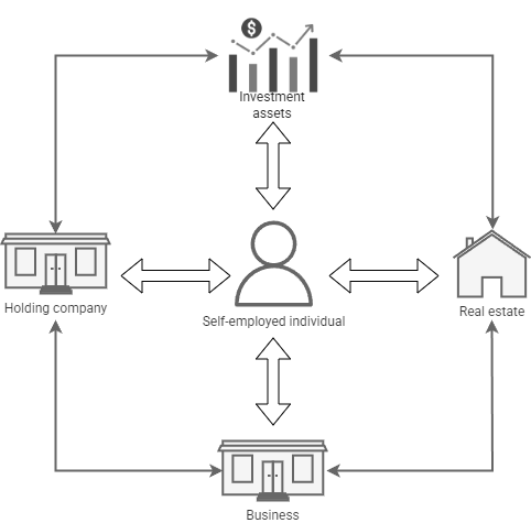
The system consists of interconnected subsystems, each with its own operational, legal, and tax regimes. Salary must be taxed privately and simultaneously reduces the profit of the business as well as retained earnings. In principle, the required cash flow can originate from salary, from the holding, from rental income, or from a mixture of these sources. Many levers can be adjusted simultaneously—but which ones are actually effective in the overall system?
In the following, several analytical steps are presented to show how such an optimization can be approached methodically. Although the presentation is sequential, the procedure is iterative: insights from one partial analysis feed back into others. The starting point is always a clear definition of the nonlinear optimization problem (NLP) and the underlying objectives.
The Nonlinear Optimization Problem (NLP) and Objectives
At present, I aim to accumulate wealth. I require cash to cover my living expenses. This is important for understanding: my living expenses are not subject to “lifestyle inflation.” I do not buy a more expensive car or take luxury trips simply because I can afford them. At the same time, I must strictly ensure that the subsystems remain liquid; insolvency must be avoided at all costs. I buffer these risks with liquidity reserves, which I refer to as “emergency funds.” The associated NLP is as follows:
Objective:
G1: ΔWealth → max
Constraints (NB):
NB1: Emergency fund (private assets) ≥ ε
NB2: Emergency fund (business) ≥ η
NB3: Emergency fund (holding) ≥ λ
NB4: CF ≥ living expenses
NB5: Living expenses ≠ f(ΔWealth, revenue, salary, distributions)
Boundary condition (RB):
RB1: Holding period of investment assets → ∞
NB1 to NB3 state that the respective emergency funds must not fall below a threshold. In practical terms, this means I always keep sufficient money in readily available accounts to cover expenses for a defined period, even if income and revenue were to cease entirely. This reflects my individual risk aversion; different life circumstances would require different thresholds. NB4 ideally prevents the emergency funds from being drawn down. NB5 explicitly guards against lifestyle inflation. RB1 is intended to protect invested capital; “buy and hold forever” is widely regarded as the long-term optimal investment strategy.
Important: objectives describe the desired system state. Costs, schedules, safety, security, quality, and similar quantities are usually constraints or boundary conditions, not objectives. Clarity in this distinction is a prerequisite for any meaningful optimization.
Equally important: every change has side effects and long-range effects. What should not change? What is currently unobtrusive but nevertheless essential is often overlooked.[1]
In the next step, we translate the initial situation and the NLP into an MDO perspective.
Multidisciplinary Design Optimization (MDO)
Figure 2 translates the system context of the underlying NLP into an MDO view.
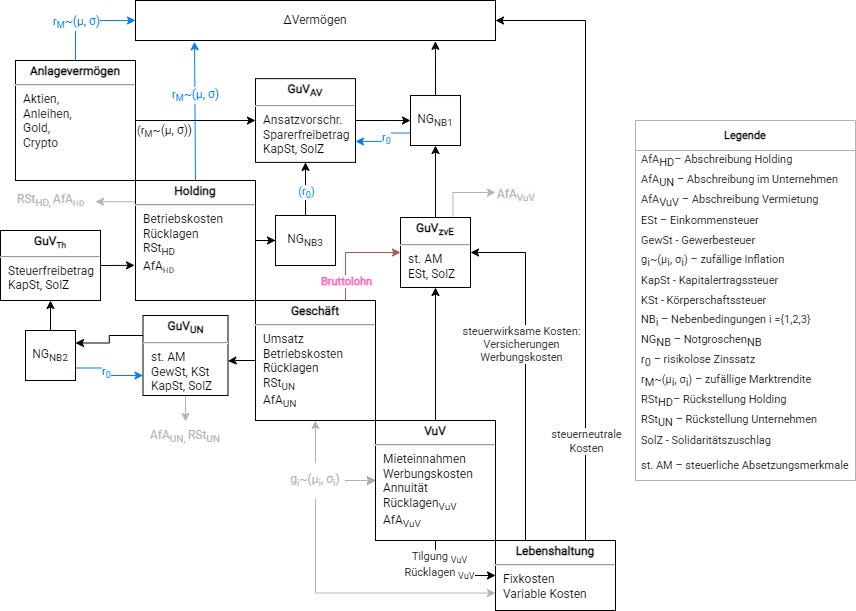
The various subsystems and their interfaces are shown. NB1 to NB3 are modeled as buffer elements. NB4 is realized by ensuring that living expenses do not receive a direct input from income sources. The interaction between taxed income and living expenses is reflected in ΔWealth. Some of these costs simultaneously affect the tax burden. It is also shown that fictitious costs such as depreciation and provisions are included in tax calculations; they have an accounting effect but do not lead to a cash outflow and are therefore eliminated again after taxation.
For the further analysis, the following variables are particularly relevant:[2]
Coupling variables that represent feedback between the subsystems.
Local variables that are required within the subsystems to transform input into output.
In practice, Systems Engineering identifies the coupling variables and derives an MDO view such as that shown in Figure 2. The disciplines are responsible for their local variables. The coupling variables thus also structure and simplify communication.
The illustration highlights the high structural and dynamic coupling of the system. An exact solution of the objective while satisfying the constraints and boundary conditions is therefore hardly practical. It would make little sense to analytically link tax formulas, profit calculation, and retained earnings in full detail. At the latest when modeling liquidity buffers, time-dependent, coupled equations would have to be formulated and optimized. Moreover, we do not want to make unrealistic simplifications: future living expenses, revenues, and market returns are uncertain and fluctuate randomly.
Let us state this clearly: instead of “everything being linked to everything,” the MDO view shows clearly delineated system parts, selected interfaces, and local parameters. Complexity is already reduced as a result. However, an exact solution of the resulting MDO is still not practically achievable.
A further reduction of complexity is required.
Isoperformance Analysis (IPA)
While the MDO view reduces the structural complexity of the system, it still allows a high combinatorial diversity of possible solutions. To further reduce this diversity, an isoperformance analysis is therefore applied.
The goal of IPA is to identify coupling variables that exhibit low sensitivity with respect to other subsystems or the system objective and can therefore be fixed.[3]
One such variable is living expenses. They are not subject to lifestyle inflation, are bounded downward by fixed costs, and do not grow arbitrarily upward. They move within a relatively narrow range and can therefore be fixed at a constant performance level (“iso”).
Accounting profits and losses of investment assets and the holding company are also fixed for the optimization, but at “zero,” and for a different reason. They can fluctuate strongly, are based on exogenous market developments, and are not subject to targeted control. Accordingly, they are unsuitable for optimization. The same applies to profit and tax calculations, which follow binding legal requirements and are not freely designable.
A look at the MDO view thus shows that, as non-fixed coupling variables, essentially only revenue and salary remain. This greatly simplifies the optimization question: which revenue–salary combination is suitable for wealth growth while covering living expenses (NB4)?
This strong simplification is specific to the system under consideration. In technical systems, a larger number of non-fixed coupling variables typically remains.
IPA reduces combinatorial diversity by fixing a satisfactory performance level for selected variables.
Nevertheless, the problem of interconnected subsystems with their respective calculation logics and tax regimes remains. This is addressed in the next step using the Swiss Army knife of quantitative analysis.
Monte Carlo Simulation (MC) of Net Cash Flow
The remaining optimization problem is translated into an MC simulation and statistically evaluated to avoid the effort of an exact analytical solution. The MC simulates different combinations of revenue, salary, and costs and their effects on net CF. The result is shown in the 3D plot in Figure 3.
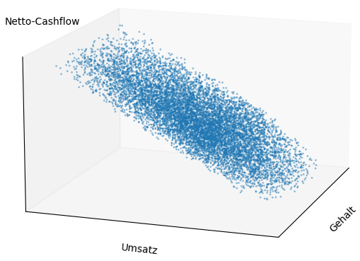
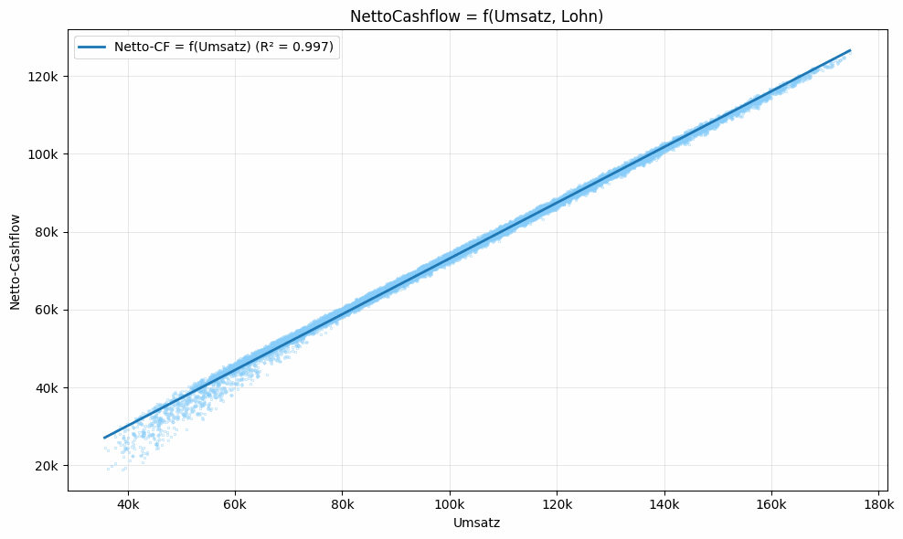
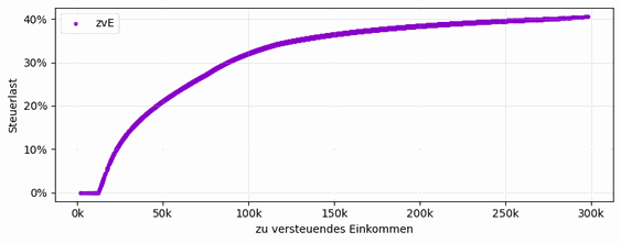
What Figure 3 does not show is noteworthy: there is neither a valley nor a peak nor a saddle point in the slanted plane. In addition, the plane runs almost parallel to the salary axis. In the projection onto revenue and net CF (Figure 4), it becomes apparent that salary has only a negligible influence. Net CF fluctuates only marginally and, according to the regression, is explained almost entirely (R² ≈ 99%) by revenue.
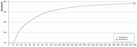
This result is surprising, since tax progression (Figure 5) suggests an optimization potential. Tax progression is also included in the simulation (Figure 6). The widespread fallacy lies in the interpretation: ratios do not represent the relevant mechanisms. Money operates in absolute amounts. Lower incomes are multiplied by lower tax factors, higher incomes by higher ones. Higher gross income therefore leads, in essence, to proportionally higher net income—the increase is merely dampened by tax deductions. This is exactly what Figure 4 shows.
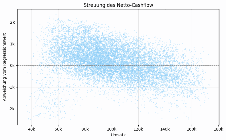
Why, then, is it so often claimed that higher gross income can even lead to lower net income? This effect also appears in the simulation. However, its magnitude is limited (Figure 7): it is mostly a matter of a few hundred euros. For low incomes this is relevant; for the system considered here, however, it does not yield any significant optimization potential, since revenues and costs are not known precisely.
Overall, the MC is consistent and allows the construction of a simple decision rule.
Conclusion: Complexity Reduction and Decision Rule
Through MDO, IPA, and MC, a substantial reduction in complexity has been achieved. The interconnected subsystems with their respective calculation logics can be reduced to a simple decision problem: for wealth growth, the specific revenue–salary combination is largely irrelevant. Lower tax outflows in the private sphere lead to higher tax outflows in the business, and vice versa. System-wide tax optimization via salary is therefore not possible. All that remains is: higher revenue helps more.
The originally complex decision problem is thus reduced to a much simpler question: how much CF is required to cover living expenses? These costs are well known and generally controllable. Extreme special cases are buffered by the emergency funds.
This assessment also holds in the long term. By means of random growth rates in the MDO, wealth and costs could be compounded in the MC and paid out with time delays. However, this does not change the conclusions as long as CF covers living expenses, these remain at a grounded level, and asset depletion is controlled via the emergency funds. All that is required is regular adjustment of the model to changed tax rules and altered life circumstances.
The approach presented is universally applicable. MDO, IPA, and MC can be used individually or in combination for various complex decision problems. In product development, for example, coupling variables would be based on physical relationships or on signal and data flows. In practice, the disciplines perform their respective MC simulations and pass the resulting coupling variables to Systems Engineering or other disciplines. In this way, work proceeds iteratively until the system-wide objective function(s) of the NLP converge.
— Yours, Nico Litschke
Endnotes
Dörner, D. (2002). The Logic of Failure: Strategic Thinking in Complex Situations (15th ed.). Reinbek near Hamburg: Rowohlt.
Agte, J., de Weck, O., Sobieszczanski-Sobieski, J., Arendsen, P., Morris, A., & Spieck, M. (2009). MDO: Assessment and direction for advancement—An opinion of one international group. Structural and Multidisciplinary Optimization, 40(1–6), 17–33. https://doi.org/10.1007/s00158-009-0381-5
de Weck, O. L., & Jones, M. B. (2006). Isoperformance: Analysis and design of complex systems with desired outcomes. Systems Engineering, 9(1), 45–61. https://doi.org/10.1002/sys.20043
Federal Ministry of Finance (BMF). (2026). Calculations and information on income tax. https://www.bmf-steuerrechner.de/ekst/eingabeformekst.xhtml